Part 2: Implementing a touch model from scratch
This is the second in a series of blog posts about typing accuracy.
- Part 1: Probable keyboard events
- Part 2: Implementing a touch model from scratch
- Part 3: Collecting touch data and re-executing touch events
- Part 4: Low end touchscreen limitations (Touching your keyboard with two fingers, no way!)
- Part 5: Test method, Results and //TODO’s
Touch (offset) model
Every person has their own way of typing and makes their own kind of mistakes. I noticed I usually hit my E key very close to the R key, which oftrn results in annoying typos. The autocorrect algorithm corrects these errors on most occasions. However, if I make too much of these errors the algorithm will have a very hard time trying to find my intended word. For every insertion, deletion or substitution the algorithm adds a penalty to the suggested word probability/score. Therefore more errors means it is less likely for the algorithm to find the word I tried to type.
The errors I make while typing depend on the situation I am in at that particular moment. When I am on my bike I tend to make a lot more errors, especially biking home after a good night out :) It would be nice if my phone learnt something from my recurring mistakes. And because the mistakes are affected by a lot of external factors, I would like a model that is personal and automagically updates based on my current ‘state’.
Implementing a model
After reading a bunch of research papers I noticed that a lot of the models had to be trained offline or required a certain amount of training data. The model I want to use should be able to be trained on the actual phone itself, preferably without any internet connection. I decided to use the touch points to estimate the parameters of a bivariate Gaussian (normal) distribution. The idea started with a paper by Antti Oulasvirta et al. where they used Gaussian distributions and calculate the distance to a key like this \(P\left( K \;\middle\vert\; T \right) = \exp (- \frac{d_k^2}{\sigma_k^2} )\) With \( d_{k} \) as the Euclidean distance of a touch point to the center of key \(k\) and \( \sigma_{k} \) as the variance of the touch point distribution around the key center. \( \sigma_{k} \) is a parameter that they estimated from training data. So for every new touch point, they calculate the probability of that touch point belonging to any given key. I am going to implement something similar however I will also use the correlation between the x and y coordinates.
Bivariate normal distributions
A nice way to visualize bivariate normal distributions is to plot their isocontours (or elevation contours). The distributions have distinctive shapes based on their parameters. The pictures below shows the three different variations.
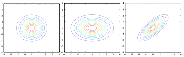
The first and leftmost variation, \( \mathbf X\sim \mathcal{N}(0,1), \mathbf Y\sim \mathcal{N}(0,1) \) and \(\rho = 0\), has the same variance for both dimensions and no correlation. It ends up looking like a circle, this means that a sample with coordinates x=0, y=1 has the same distance to the distribution as a sample with coordinates x=1, y=0.
The second variation, \( \mathbf X\sim \mathcal{N}(0,2), \mathbf Y\sim \mathcal{N}(0,1) \) and \(\rho = 0\), is axis aligned but the variance is different for both dimensions, now it ends up looking like an ellipse. The two samples in the previous example have a different distance to the distribution as the variance of both dimensions is different.
The third and last version, \( \mathbf X\sim \mathcal{N}(0,1), \mathbf Y\sim \mathcal{N}(0,1) \) and \(\rho = 0.75\), is not axis aligned, which means the two dimensions are correlated, and the isocontours look like a rotated ellipse.
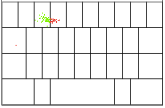
Explaining the dataset
The dataset used in this example consists of annotated data collected from users typing on the gaia keyboard. The users had to type fixed sentences, therefore the intended touch targets are known. For every touch we have information about the x and y coordinates and the key they intended to hit. The figure below shows an example of recorded data for the key E, where green dots were ‘on target’ and red points missed the intended key. More on the dataset here
Use samples to estimate normal distribution parameters
For each of the N keys we will estimate the parameters of a multivariate normal distribution. Given this set of N distributions and one new touch point T we can calculate which key is the most probable intended target. To do so we need to use some kind of distance measure. The measure we will use is the Mahalanobis distance as it takes correlation between dimensions into account. The Mahalanobis distance is defined as \(D_m(x) = \sqrt{(x-\mu)^T S^{-1} (x-\mu)}\)
Parameter estimation
To estimate the parameters of a key distribution we use annotated touch events, these events have been classified to belong to a certain key. These annotated touch events, which we will call samples, will be used to estimate the mean, variance and covariance of a distribution for a given key. To build a model which updates itself based on the last touch events, we could use a FIFO queue to keep track of the last 50 touches for every key. When we estimate the distribution parameters based on the FIFO queue, we have a model which updates itself according to the user, the device and the users’ state. The size of the FIFO queue determines how fast the model changes given the most recent touches. Lets take a look how we can estimate the distribution parameters given an arbitrary amount of samples.
Each sample point holds a value for the two dimensions x and y
	var Sample = (function () {
	    function Sample(x, y) {
	        this.x = x;
	        this.y = y;
	    }
	    Sample.prototype.subtract = function (p) {
	        return new Sample(this.x - p.x, this.y - p.y);
	    };
	    return Sample;
	})();
First we need the sample mean \(\mu\) (or \(\bar{s}\)) which is a vector containing the average for both dimensions \(\mu = \frac{1}{N} \sum_{i=1}^N s_i\)
	function mean(samples){
		// samples is an array of samples

	    var mean = new Sample(0, 0),
	    	N = samples.length;

	    // take the sum of all samples
	    for (var i = 0; i < N; i++) {
	        mean.x += samples[i].x;
	        mean.y += samples[i].y;
	    }

	    // now divide by the amount of samples to get the mean/avg
	    mean.x = mean.x / N;
	    mean.y = mean.y / N;
	    return mean;
	}
To calculate the inverse covariance matrix \(S^{-1}\) we first need to build the covariance matrix \(S\). Lets start by calculating the variance. Variance is a measure that is used to determine how far points are spread out. \(\sigma^2 = \frac{1}{N-1} \sum_{i=1}^N (x_i - \mu)\) In this example we calculate the variance for both dimensions on one loop
	function variance(samples){
		var mean = this.mean(samples),
			variance = new Sample(0, 0),
			N = samples.length,
			dx,dy;
		for (var i = 0; i < N; i++) {
			dx = samples[i].x - mean.x;
			dy = samples[i].y - mean.y;
		    variance.x += dx * dx;
		    variance.y += dy * dy;
		}
		variance.x = variance.x / (N - 1);
		variance.y = variance.y / (N - 1);
		return variance;
	}
Now we are going to calculate the unbiased sample covariance
\(\hat{S} = \frac{1}{N-1} \sum_{i=1}^N (x_i - \mu) (x_i - \mu)'\)
	function covariance(samples){
		var mean = this.mean(samples),
			covariance = 0,
			N = samples.length;
	    for (var i = 0; i < N; i++) {
	        covariance += (samples[i].x - mean.x) * (samples[i].y - mean.y);
	    }
	    covariance = covariance / (N - 1);
	    return covariance;
	}
We can calculate variance for both dimensions and the covariance in one go
With the variance and the covariance calculated, we have the covariance block matrix: \(S_{X,Y} = \begin{bmatrix} S_{XX} & S_{XY} \\\\ S_{YX} & S_{YY} \end{bmatrix}\) \(S_{XX}\) is the variance of the samples in the X dimension, \(S_{YY}\) is the variance of samples in the Y dimension and \(S(XY)\) and \(S(YX)\) is the sample covariance we just calculated.
Just one more step is needed to be able to calculate the inverse matrix \(S^{-1}\), as we need the determinant of the covariance matrix \(\left|S\right|\). The determinant for a 2D matrix can be calculated by \(\left|A\right| = a d - b c\) with \(A = \bigl(\begin{smallmatrix} a & b \\ c & d\end{smallmatrix} \bigr)\).
	function getDeterminant(covarianceMatrix) {
        // matrix = [a b; c d]
        // determinant = ad - bc
        return covarianceMatrix[0][0] * covarianceMatrix[1][1] - covarianceMatrix[0][1] * covarianceMatrix[1][0];
    };
Now we have calculated everything we need for the inverse matrix, fortunately we only use two dimensions and can calculate the inverse matrix pretty easily (extra free comic sans math).
	function getInverseMatrix(matrix, determinant) {
        // Input matrix = A = [a b; c d] = [varX cov; cov varY]
        // Inverse matrix = A^-1 = [? ?;? ?]
        // Identity matrix = I = [1 0; 0 1]
        // Where A * A^-1 = I
        // Steps:
        // A^-1 = 1/determinant(A) * adjugate(A)
        // adjugate(A) = [d -b; -c a] = [varY -cov; -cov varX]
        if (matrix.length !== 2 || matrix[0].length !== 2 || matrix[1].length !== 2)
            throw new Error('Expected a 2 by 2 input matrix');
        if (matrix[0][1] !== matrix[1][0])
            throw new Error('Expected input matrix: [varX cov; cov varY]');
        if (!determinant)
            determinant = this.getDeterminant(matrix);
        if (determinant === 0)
            throw new Error('Inverse matrix does not exist if determinant is 0');

        var inverseMatrix = [];
        inverseMatrix[0] = [];
        inverseMatrix[1] = [];
        //Take negative
        inverseMatrix[0][1] =
        inverseMatrix[1][0] = -matrix[0][1] / determinant;
        //swap a and d
        inverseMatrix[0][0] = matrix[1][1] / determinant;
        inverseMatrix[1][1] = matrix[0][0] / determinant;
        return inverseMatrix;
    }
Finally we can calculate the distance between a new sample and a distribution! Given the sample, mean and inverse matrix we can use the definition for the Mahalanobis distance \(D_m(x) = \sqrt{(x-\mu)^T S^{-1} (x-\mu)}\)
	 function mahalanobis(sample, mean, inverseMatrix) {
        // Subtract mu from given coordinate
        // s = (x - mu) = [x y]-[muX muY]
        var s = sample.subtract(mean);

        //  Multiply the inversematrix by s and s'
        //  (x - mu)' * S^-1 * (x - mu)
        var radicand =  s.x * (inverseMatrix[0][0] * s.x + inverseMatrix[0][1] * s.y) +
                 		s.y * (inverseMatrix[1][0] * s.x + inverseMatrix[1][1] * s.y);

        return Math.sqrt(radicand);
    };
The multiplication does look a bit ugly, but I did not feel like using a vector/matrix lib in order to do one simple multiplication
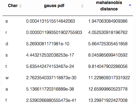
Which key did we intend to touch?
For every key we estimated the distribution parameters. For every new sample (touch event) we can calculate the distance to those key distributions. The key with the smallest distance will be selected as intended target. Note that the touch coordinates do not necessarily have to be within the key boundaries.
Instead of picking one most probable touch target we could also use the distance to the keys to estimate the probability that this touch event belongs to a certain key. These probabilities could be used to assist the autocorrect algorithm. For example by sending a map with keys and corresponding probabilities instead of one distinct key as input.